This is an example and tutorial of setting up a 2D gmsh input file for compressible flow with LODI extruded boundaries. The tutorial provides guidance/examples on creating the gmsh mesh using the GUI.
Geometry
- Install Gmsh and open a new document
-
Define the outline of the pipe using a series of points under
Modules > Geometry > Elementary entities > Add > Point- 0.0, 0.0, 0.0
- 0.5, 0.0, 0.0
- 0.5, .1, 0.0
- 0.0, .1, 0.0
-
Connect the points using
Modules > Geometry > Elementary entities > Add > Line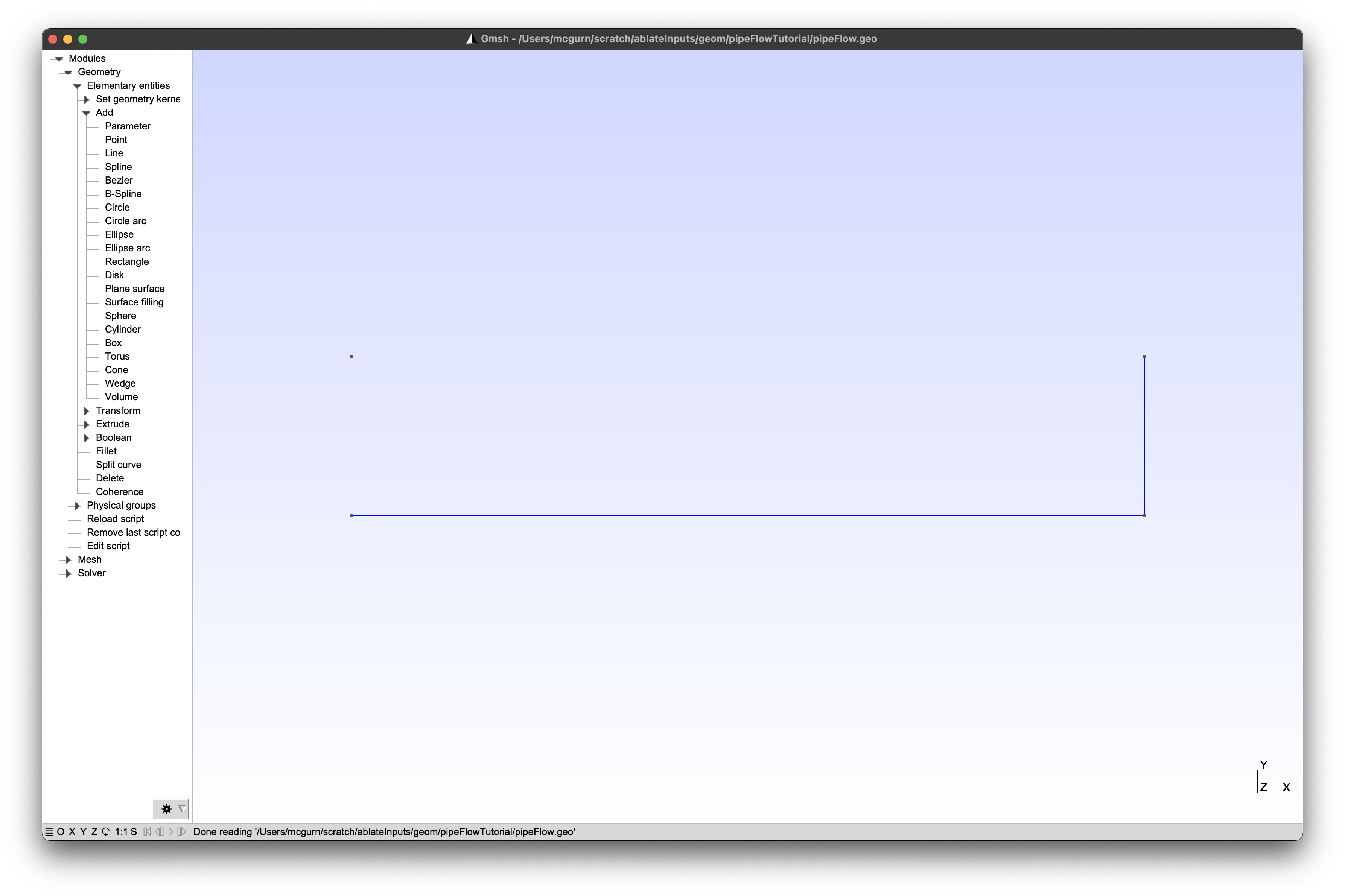
-
Define a new surface using
Modules > Geometry > Elementary entities > Add > Plane surface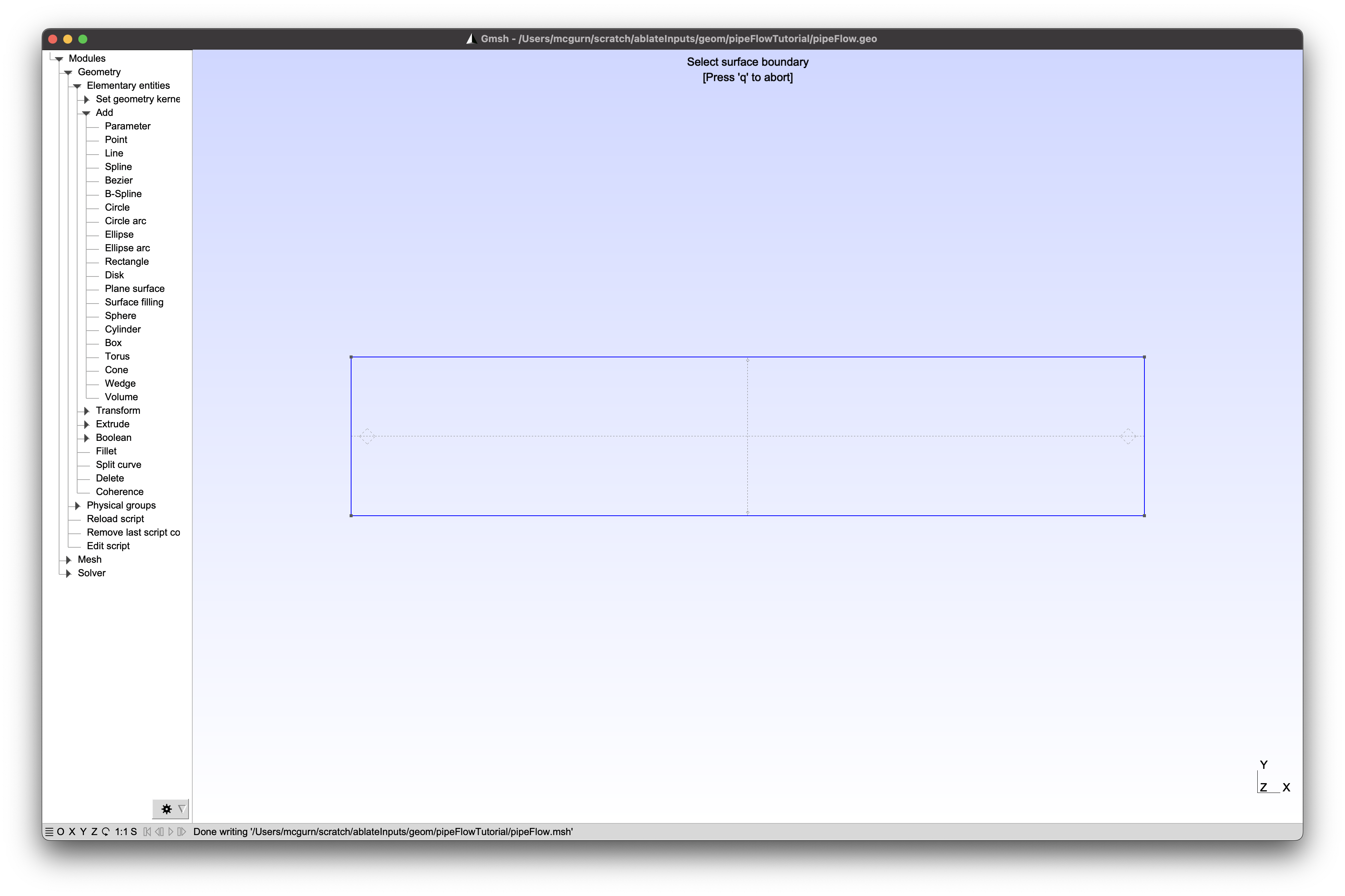
-
Define the boundary conditions using physical groups. Define the left boundary as
inletusingModules > Geometry > Physical groups > Add > Curve. Repeat for thewall(top/bottom) andoutlet(right hand side). - Define the
mainmesh using a physical group. Define the surface asmainusingModules > Geometry > Physical groups > Add > Surface.
Meshing
-
Configure Gmsh to produce hexes/quads using the following settings in
Tools > Options > Mesh > General Tabsetting value 2D algorithm Frontal-Delaunay for Quads (experimental) 3D algorithm Delaunay 2D recombination algorithm Blossom Full-Quad Recombine all triangular meshes checkSubdivision algorithm All Quads Min/Max element size Reasonable values for mesh 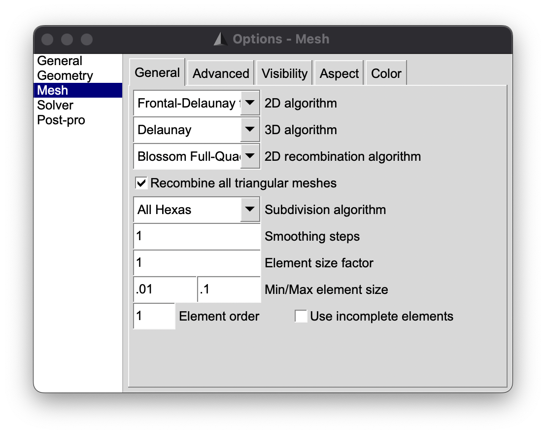
- Generate the mesh
- Generate the line mesh
Modules > Mesh > 1D - Generate the surface mesh
Modules > Mesh > 2D - If creating a 3D mesh,
Modules > Mesh > 3D - If a higher resolution mesh is needed, adjust the settings in Step 1 or select
Modules > Mesh > Refine by splitting
- Generate the line mesh
- Output the mesh.
File > Save Meshshould produce a *.msh file with the same name as the geometry. The pipeFlow.geo pipeFlow.msh files used in this example are provided to download.
compressibleFlow/gmshPipeFlow.yaml
---
test:
  # a unique test name for this integration tests
  name: gmshPipeFlow
  # run mpi with two ranks
  ranks: 2
  # create a default assert that compares the log file
  assert: "inputs/compressibleFlow/gmshPipeFlow/gmshPipeFlow.txt"

# metadata for the simulation
environment:
  title: _gmshPipeFlow
  tagDirectory: false
# global arguments that can be used by petsc
arguments:
  # The gmsh arguments must be global because they are used before the mesh options are parsed
  dm_plex_gmsh_use_regions: true
# set up the time stepper responsible for marching in time
timestepper:
  # time stepper specific input arguments
  arguments:
    ts_type: rk
    ts_max_time: 100000
    ts_max_steps: 50
    ts_dt: 1.0E-10
    ts_adapt_safety: 0.9
    ts_adapt_type: physicsConstrained
  # io controls how often the results are saved to a file for visualization and restart
  io:
    interval: 5 # results are saved at every 5 steps.  In real simulations this should be much larger.
  # load in the gmsh produced mesh file
  domain: !ablate::domain::MeshFile
    path: pipeFlow.msh
    options:
      dm_plex_check_all: true
      dm_distribute: false # turn off default dm_distribute so that we can extrude label first
    # specify any modifications to be performed to the mesh/domain
    modifiers:
      - # GMsh/dm_plex_gmsh_use_regions creates individual labels with their separate values. By collapsing the labels to the default values
        # this input file does not need to individually specify each one for boundary conditions
        !ablate::domain::modifiers::CollapseLabels
        regions:
          - name: inlet
          - name: wall
          - name: outlet
          - name: main
      -  # use the newly collapsed labels to extrude the boundary.  Do not extrude the cell
        !ablate::domain::modifiers::ExtrudeLabel
        regions:
          - name: inlet
          - name: wall
          - name: outlet
        # mark all the resulting boundary faces with boundaryFaces label
        boundaryRegion:
          name: boundaryFaces
        # tag the original mesh as the flow region
        originalRegion:
          name: flowRegion
        # tag the new boundary cells for easy boundary condition specifications
        extrudedRegion:
          name: boundaryCells
      # it may be helpful to print the dm and labels to debug
      #- !ablate::monitors::DmViewFromOptions
      #  options: ":$OutputDirectory/pipeFlow.tex:ascii_latex"
      #- !ablate::monitors::DmViewFromOptions
      #  options: ascii::ascii_info_detail
      # if using mpi, this modifier distributes cells
      - !ablate::domain::modifiers::DistributeWithGhostCells
        ghostCellDepth: 2

    fields:
      # all fields must be defined before solvers.  The ablate::finiteVolume::CompressibleFlowFields is a helper
      # class that creates the required fields for the compressible flow solver (rho, rhoE, rhoU, ...)
      - !ablate::finiteVolume::CompressibleFlowFields
        eos: !ablate::eos::PerfectGas &eos
          parameters:
            gamma: 1.4
            Rgas: 287.0
          # species are added to the flow through the eos.  This allows testing of the species transport equations
          species: [ N2, H2O, O2 ]
      # by adding a pressure field the code will compute and output pressure
      - name: pressure
        location: AUX
        type: FVM
  # set the initial conditions of the flow field
  initialization:
    # The ablate::finiteVolume::CompressibleFlowFields is a helper
    # class that creates the required fields for the compressible flow solver (rho, rhoE, rhoU, ...)
    - !ablate::finiteVolume::fieldFunctions::Euler
      state:
        &flowFieldState
        eos: *eos
        pressure: 101325.0
        temperature: 300
        velocity: "0.0, 0.0"
        # individual mass fractions must be passed to the flow field state to compute density, energy, etc.
        other: !ablate::finiteVolume::fieldFunctions::MassFractions
          eos: *eos
          values:
            - fieldName: N2
              field: "x > .1 ? .2 : 1.0"
            - fieldName: H2O
              field: " x> .1 ? .3 :0"
            - fieldName: O2
              field: " x > .1 ? .5 : 0"
    # the same state can be used to internalize the DensityMassFractions field from density and mass fractions
    - !ablate::finiteVolume::fieldFunctions::DensityMassFractions
      state: *flowFieldState

# solvers can be combined
solvers:
  # The compressible flow solver will solve the compressible flow equations over the interiorCells
  - !ablate::finiteVolume::CompressibleFlowSolver
    id: vortexFlowField
    # only apply this solver to the flowRegion, area without faces
    region:
      name: flowRegion
    additionalProcesses:
      - !ablate::finiteVolume::processes::PressureGradientScaling
        &pgs
        eos: *eos
        alphaInit: 100.0
        maxAlphaAllowed: 100.0
        domainLength: 0.165354
        log: !ablate::monitors::logs::CsvLog
          name: pgsLog

    # a flux calculator must be specified to so solver for advection
    fluxCalculator: !ablate::finiteVolume::fluxCalculator::AusmpUp
      pgs: *pgs

    # the default transport object assumes constant values for k, mu, diff
    transport:
      k: .2
      mu: .1
      diff: 1E-4

    # cfl is used to compute the physics time step
    parameters:
      cfl: 0.5

    # share the existing eos with the compressible flow solver
    eos: *eos

    monitors:
      # output the timestep and dt at each time step
      - !ablate::monitors::TimeStepMonitor
        interval: 10

  # use a boundary solver to update the cells in the gMsh inlet region to represent an inlet
  - !ablate::boundarySolver::BoundarySolver
    id: inlet
    region:
      name: inlet
    fieldBoundary:
      name: boundaryFaces
    mergeFaces: false
    processes:
      - !ablate::boundarySolver::lodi::Inlet
        eos: *eos
        pgs: *pgs
        velocity: "min(10, 10*t), 0" # for stability, increase the velocity slowly

  # use a boundary solver to update the cells in the gMsh outlet region to represent an open pipe
  - !ablate::boundarySolver::BoundarySolver
    id: openBoundary
    region:
      name: outlet
    fieldBoundary:
      name: boundaryFaces
    mergeFaces: true
    processes:
      - !ablate::boundarySolver::lodi::OpenBoundary
        eos: *eos
        reflectFactor: 0.0
        referencePressure: 101325.0
        maxAcousticsLength: 1
        pgs: *pgs

  # use a boundary solver to update the cells in the wall region to represent standard wall
  - !ablate::boundarySolver::BoundarySolver
    id: wall
    region:
      name: wall
    fieldBoundary:
      name: boundaryFaces
    mergeFaces: true
    processes:
      - !ablate::boundarySolver::lodi::IsothermalWall
        eos: *eos
        pgs: *pgs